What is Central Limit Theorem (CLT) in Statistics : The Foundation of Modern Statistics Behind Six Sigma, Quality Engineering & Data Analysis
At first glance, real-world data can appear unpredictable, messy, and difficult to analyze. Yet many of the statistical methods used in Six Sigma, Quality Engineering, Process Capability Analysis, SPC, hypothesis testing, and data analytics rely on a surprisingly powerful principle that brings order to this randomness: the Central Limit Theorem (CLT).
The Central Limit Theorem is one of the most important concepts in statistics because it explains why sample data can be used to make reliable conclusions about larger populations. It provides the mathematical foundation for many of the tools and techniques that quality professionals, engineers, researchers, and data analysts use every day to make decisions under uncertainty.
Whether you’re calculating confidence intervals, performing statistical tests, analyzing process performance, or interpreting quality data, understanding the Central Limit Theorem helps explain why these methods work and why statistics remains such a powerful tool for solving real-world problems.
What is the Central Limit Theorem?
Have you ever wondered how companies confidently make decisions about millions of products after inspecting only a few hundred? Or how election agencies can predict the outcome of a national election by surveying just a small percentage of voters? The answer lies in one of the most important concepts in statistics—the Central Limit Theorem (CLT).
The Central Limit Theorem states that when sufficiently large random samples are repeatedly drawn from a population, the distribution of the sample means approaches a normal (bell-shaped) distribution regardless of the shape of the original population distribution.
When I first started learning statistics during my Six Sigma journey, I memorized the definition of the Central Limit Theorem because it appeared in almost every textbook and certification exam. I knew the words, but I didn’t truly understand why the theorem was so important. It wasn’t until I began working on real manufacturing and quality engineering projects that its significance became clear. Whether we were evaluating process capability, analyzing product measurements, performing hypothesis tests, or making decisions from production data, the Central Limit Theorem was quietly working behind the scenes. I realized that CLT isn’t just another statistical formula to remember—it’s the reason we can confidently make decisions using samples instead of measuring every single item.
In simple terms, the Central Limit Theorem explains what happens when we repeatedly collect random samples from a population and calculate the average of each sample. Even if the original population is highly skewed, irregular, or does not follow a normal distribution, the distribution of those sample averages gradually becomes approximately normal (bell-shaped) as the sample size increases, provided certain conditions are met. This predictable behavior is what allows statisticians, engineers, researchers, and data analysts to apply powerful statistical techniques to real-world problems.
What makes the Central Limit Theorem truly fascinating is that it works across an astonishing variety of situations. The original data does not have to resemble a bell curve. It could represent customer waiting times, manufacturing defects, online shopping transactions, hospital recovery times, website response times, or daily rainfall measurements. Despite these very different types of data, the averages of sufficiently large random samples tend to follow the familiar normal distribution. This consistency is one of the reasons the theorem is considered a cornerstone of modern statistics.
One of the biggest misconceptions about the Central Limit Theorem is that it says the original data must be normally distributed. This is not true. The theorem does not transform your population data into a normal distribution. Instead, it describes the behavior of the sampling distribution of the sample mean. This distinction is often overlooked by beginners, yet understanding it is essential for correctly applying statistical methods.
The importance of the Central Limit Theorem extends far beyond the classroom. It forms the statistical foundation for confidence intervals, hypothesis testing, regression analysis, process capability studies, Statistical Process Control (SPC), Six Sigma methodologies, and many machine learning algorithms. In other words, much of modern data analysis depends on this single principle. Without it, drawing reliable conclusions from sample data would be far more difficult, and many of the analytical tools we use every day would lose their statistical justification.
Throughout this article, we’ll move beyond memorizing definitions. You’ll learn why the Central Limit Theorem works, when it applies, how it supports Six Sigma and quality engineering, and where it is used in real-world decision-making. By the end, you’ll not only understand the theorem—you’ll also recognize why it has earned the reputation as the foundation of modern statistics.
Understanding Population vs Sample
Before we dive deeper into the Central Limit Theorem, we need to understand two ideas that quietly sit behind almost every statistical calculation: population and sample. These terms may sound basic, but they form the foundation of confidence intervals, hypothesis testing, process capability analysis, control charts, Six Sigma projects, and many other statistical tools. In fact, the Central Limit Theorem only makes sense once you understand how a sample relates to the population it represents.
Let’s start with a simple question. Imagine a factory produces one million precision components each month. If the quality team wants to know the average diameter of all those components, the most accurate approach would be to measure every single part. That complete collection of components is what statisticians call the population. A population is simply the entire group we want to study or make conclusions about. Depending on the situation, it could mean every product manufactured during a specific period, every customer who purchased a product, all patients in a clinical study, or every transaction processed by a business.
The challenge, of course, is that studying an entire population is often impractical. Measuring one million parts would require enormous amounts of time, labor, and cost. In some industries, it may not even be possible. During my years working in manufacturing and medical device environments, I rarely encountered situations where every product could be inspected. In many cases, testing itself was expensive, time-consuming, or partially destructive. Instead, we selected a carefully planned subset of products, performed detailed measurements, and used those results to understand how the overall process was performing. That smaller subset is known as the sample.
A sample is not valuable simply because it is smaller. Its value comes from its ability to represent the larger population. When a sample is selected properly, it can tell us surprisingly accurate things about the population from which it came. This is one of the most powerful ideas in statistics. Rather than examining every observation, we can study a relatively small amount of data and still make informed decisions about a much larger group.
I often explain this concept using a simple example outside of manufacturing. Imagine preparing a large pot of soup. Before serving it, you probably take one spoonful to check the taste. You don’t drink the entire pot. If the soup has been mixed well, that single spoonful provides a good indication of the flavor of the whole pot. Statistics works in much the same way. The spoonful represents the sample, while the entire pot represents the population. The quality of the conclusion depends on whether the sample truly represents what is happening in the larger group.
This idea applies everywhere, not just in factories. Election polls do not interview every voter. Hospitals do not test a new treatment on every patient before evaluating its effectiveness. Businesses rarely contact every customer when measuring satisfaction. Even online platforms that analyze user behavior rely heavily on samples rather than complete datasets. Across industries, decisions are regularly made using samples because studying the entire population would be either too expensive, too slow, or simply impossible.
However, there is an important catch. Not every sample tells the truth about the population. Over the years, I’ve seen teams collect data that looked impressive on paper but led to poor decisions because the sample wasn’t truly representative. Imagine measuring parts from only one machine when several machines produce the same product. Or collecting data from only the day shift while ignoring the night shift. The calculations may be mathematically correct, but the conclusion can still be misleading because the sample fails to reflect the broader process. Statistics cannot completely compensate for poor data collection.
The distinction between population and sample becomes especially important in Six Sigma projects. During the Measure and Analyze phases, we rarely work with population data. Instead, we collect a sample and use it to estimate what is happening in the larger process. The goal is not to describe the sample itself but to draw meaningful conclusions about the population. This is where statistics becomes truly powerful. It allows us to move from a limited amount of data to informed business decisions.
The Central Limit Theorem provides the bridge between sample data and population-level conclusions. It helps explain why sample averages behave in a predictable way and why statisticians, researchers, quality professionals, and data analysts can confidently use sample data to make decisions about much larger populations. Once you understand the relationship between population and sample, you’re ready to see why the Central Limit Theorem is often described as the statistical engine powering modern data-driven decision making.
🎓 Top-Rated Courses & Certifications
Try changing your filters or searching for another course.
Why is the Central Limit Theorem important?
If someone asked me to identify the single most important concept in applied statistics, the Central Limit Theorem (CLT) would be at the top of my list. That may sound surprising, but after years of working in quality engineering, medical devices, and Six Sigma projects, I’ve realized that many statistical tools we use every day quietly depend on this one principle. Early in my career, I regularly used software like Minitab to perform hypothesis tests, calculate confidence intervals, analyze process capability, and interpret production data. At the time, these seemed like completely different techniques. It wasn’t until I understood the Central Limit Theorem that I realized they all shared the same statistical foundation. From that moment, statistics stopped feeling like a collection of formulas and started making logical sense.
The importance of the Central Limit Theorem comes from a simple reality: we rarely have access to an entire population. Manufacturers cannot inspect every product, hospitals cannot evaluate every patient, and researchers cannot collect data from every possible subject. Instead, decisions must be made using carefully selected samples. The challenge is determining whether those samples truly represent the larger population. The Central Limit Theorem provides the statistical confidence to make that connection, allowing us to draw reliable conclusions from limited data.
I experienced this firsthand while working on manufacturing and process improvement projects. Thousands of components were produced during each production run, making it impossible to measure every single part. Instead, engineers collected random samples to monitor quality, evaluate process stability, and determine whether corrective actions were necessary. At first, I accepted this approach because it was standard practice. Later, I began asking a more important question: Why should a few dozen measurements tell us anything about thousands of products? The answer wasn’t based on experience or guesswork—it was based on the Central Limit Theorem.
One of the reasons CLT is so powerful is that it brings predictability to unpredictable data. Real-world data is rarely perfect. Manufacturing measurements may be skewed, customer waiting times may vary widely, and financial or healthcare data often contains unexpected variation. Yet, when random samples are collected correctly, the averages of those samples follow a predictable pattern. This allows statisticians, engineers, researchers, and analysts to apply methods such as confidence intervals, hypothesis testing, regression, Statistical Process Control (SPC), and process capability analysis with confidence.
The influence of the Central Limit Theorem extends far beyond manufacturing. Healthcare researchers use it to evaluate new treatments, polling organizations rely on it to estimate election results, financial analysts assess market trends with sampled data, and data scientists build predictive models using representative datasets. Although these fields appear very different, they all face the same challenge—making informed decisions about a large population using only a sample. The Central Limit Theorem makes those decisions statistically sound.
For me, the real value of the Central Limit Theorem became clear when I stopped treating it as a definition to memorize for certification exams and started seeing it as the invisible engine behind statistical decision-making. Once you understand its role, concepts like confidence intervals, hypothesis testing, process capability, control charts, and Six Sigma are no longer isolated topics—they become part of the same statistical framework. That’s why the Central Limit Theorem is widely regarded as one of the most important ideas in modern statistics. It transforms sample data into reliable knowledge, helping organizations make better decisions with confidence rather than guesswork.
Why is CLT Called the Foundation of Modern Statistics?
When I first started learning statistics, I often felt like I was studying a collection of unrelated topics. One chapter discussed confidence intervals, another focused on hypothesis testing, then came control charts, process capability, regression, and Six Sigma analysis. Each topic seemed to have its own formulas, rules, and terminology. It wasn’t until I began applying statistics to real manufacturing and quality improvement projects that I noticed a common thread running through many of these methods. Behind the calculations and software outputs was the same fundamental idea: using a sample to understand a much larger population. That idea is exactly why the Central Limit Theorem (CLT) is often called the foundation of modern statistics.
The reason is surprisingly simple. In the real world, we rarely have the luxury of collecting data from an entire population. A manufacturer cannot inspect every product, a hospital cannot study every patient, and a business cannot survey every customer. Decisions must be made using limited data. The challenge is determining whether that sample data is reliable enough to represent the bigger picture. The Central Limit Theorem provides the statistical bridge that makes this possible. It explains why sample averages behave predictably and why conclusions drawn from well-designed samples can be trusted.
I experienced this firsthand throughout my career in manufacturing and medical device industries. Production lines often generated thousands of parts every day, yet quality decisions were typically based on relatively small samples collected at defined intervals. Engineers used those measurements to assess process stability, monitor product quality, and determine whether corrective action was needed. At first, I accepted this as standard practice. Later, I began asking a more important question: Why should a small sample tell us anything meaningful about thousands of products? The answer led directly back to the Central Limit Theorem. Once I understood that principle, statistical methods stopped feeling like black-box calculations and started feeling far more logical and trustworthy.
What makes CLT so powerful is its ability to bring structure to messy real-world data. Manufacturing measurements, customer wait times, defect counts, and business metrics rarely follow perfect textbook distributions. Despite that reality, the averages of sufficiently large random samples tend to behave in a predictable and approximately normal way. That predictable behavior is what allows statisticians, engineers, researchers, and analysts to estimate population values, measure uncertainty, and make data-driven decisions with confidence.
If you look closely, you’ll find the Central Limit Theorem working behind many of the most widely used statistical techniques. Confidence intervals, hypothesis tests, Statistical Process Control (SPC), process capability analysis, Six Sigma projects, business analytics, healthcare research, and even many data science applications all depend on understanding how sample statistics behave. Although these methods may appear different on the surface, they share the same foundation.
For me, the easiest way to think about the Central Limit Theorem is as the engine that powers statistical inference. It transforms sample data into meaningful insight. It allows organizations to make informed decisions without measuring every observation. Most importantly, it gives us a rational way to quantify uncertainty rather than relying on assumptions or intuition alone.
That is why the Central Limit Theorem has earned its reputation as the foundation of modern statistics. It is not simply another theorem to memorize for an exam. It is the principle that connects data to decisions, samples to populations, and uncertainty to confidence. Once you understand its role, many statistical concepts that once seemed independent suddenly fit together as part of a much larger picture. In many ways, modern statistics is built on this single idea—and that is precisely what makes the Central Limit Theorem so important.
How the Central Limit Theorem Works (Visual Explanation)
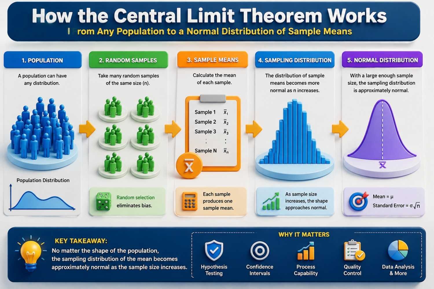
One of the easiest ways to understand the Central Limit Theorem is to see it visually. Instead of starting with formulas, the diagram below shows how random samples taken from almost any population can eventually produce a bell-shaped distribution of sample means. This simple but powerful idea explains why statisticians, quality engineers, and data analysts can make reliable decisions using a sample rather than measuring an entire population.
Central Limit Theorem Formula & Mathematical Explanation
Central Limit Theorem Formula
When I first learned the Central Limit Theorem, I treated the formula like something to memorize for exams. I could write the equation correctly, but if someone asked me what each symbol meant or why it mattered, I struggled to answer. Everything changed when I started applying statistics to real manufacturing and Six Sigma projects. I realized the formula wasn’t just mathematics—it explained why engineers and analysts can confidently make decisions using only a sample instead of an entire population. Since then, I’ve always encouraged learners to understand the logic behind the equation, not just memorize it.
The Central Limit Theorem states that if we repeatedly draw random samples of the same size from a population and calculate the mean of each sample, the distribution of those sample means approaches a normal (bell-shaped) distribution as the sample size becomes sufficiently large. This relationship is expressed mathematically as:
Although the equation may look intimidating at first, each symbol has a simple meaning. Here, Xˉ represents the sample mean, μ is the population mean, σ is the population standard deviation, n is the sample size, and nσ is the Standard Error (SE), which measures how much the sample means are expected to vary from one sample to another.
Standard Error Formula
The first equation tells us that the average of all possible sample means equals the population mean, which means properly collected samples are centered around the true population value. The second equation introduces the Standard Error, one of the most practical concepts in applied statistics. Unlike the standard deviation, which measures the variation of individual observations, the Standard Error measures the variation of sample averages. The smaller the Standard Error, the closer those sample averages are likely to be to the true population mean.
For example, suppose a process has a population mean of 100, a population standard deviation of 12, and a sample size of 36.This means that although individual observations may vary considerably, the sample means typically vary by only about 2 units around the population mean. This reduction in variability is the reason sample averages are so powerful in quality engineering, Six Sigma, and statistical decision-making.
Perhaps the most remarkable aspect of the Central Limit Theorem is that it works even when the original population is not normally distributed. Manufacturing measurements, service times, customer transactions, and many real-world datasets are often skewed or irregular. Yet as the sample size increases, the distribution of sample means becomes increasingly normal and predictable. This predictable behavior is what makes confidence intervals, hypothesis testing, Statistical Process Control (SPC), process capability analysis, and many other statistical techniques possible.
The most important lesson isn’t the equation itself—it’s what the equation represents. The Central Limit Theorem explains why larger samples provide more reliable estimates and why a relatively small amount of data can reveal meaningful information about a much larger population. Once you understand that idea, the formula stops being something to memorize and becomes one of the most practical tools in statistics.
Key Insights
- Mean of the sampling distribution = Population Mean (μ\muμ)
- Standard Deviation of the sampling distribution = Standard Error (σ/n\sigma/\sqrt{n}σ/n)
- As sample size increases, the Standard Error decreases.
- Larger samples provide more reliable estimates of the population mean.
📚 Recommended Books for Professionals
Try removing one or more filters.
Conditions & Assumptions
- Random Sampling
Every observation should have an equal chance of being selected.
Random sampling helps ensure the sample represents the entire population.
Non-random samples can introduce bias and produce misleading conclusions. - Independent Observations
Each observation should be independent of the others.
One measurement should not influence another.
Repeatedly measuring the same item does not create independent observations. - Adequate Sample Size
The sample size should be sufficiently large.
n ≥ 30 is a common rule of thumb, but it is not a universal requirement.
Highly skewed or heavy-tailed populations often require larger sample sizes.
If the population is already normally distributed, smaller samples may be sufficient. - Finite Mean and Variance
The population should have a finite mean and finite variance.
This assumption is satisfied in almost all practical applications, including manufacturing, healthcare, engineering, business, and finance. - CLT Applies to Sample Means
The theorem describes the distribution of sample means, not the distribution of the original data.
The population itself does not need to follow a normal distribution.
Even if the original data is skewed, the sampling distribution of the mean becomes approximately normal as the sample size increases.
Sample Size Requirements
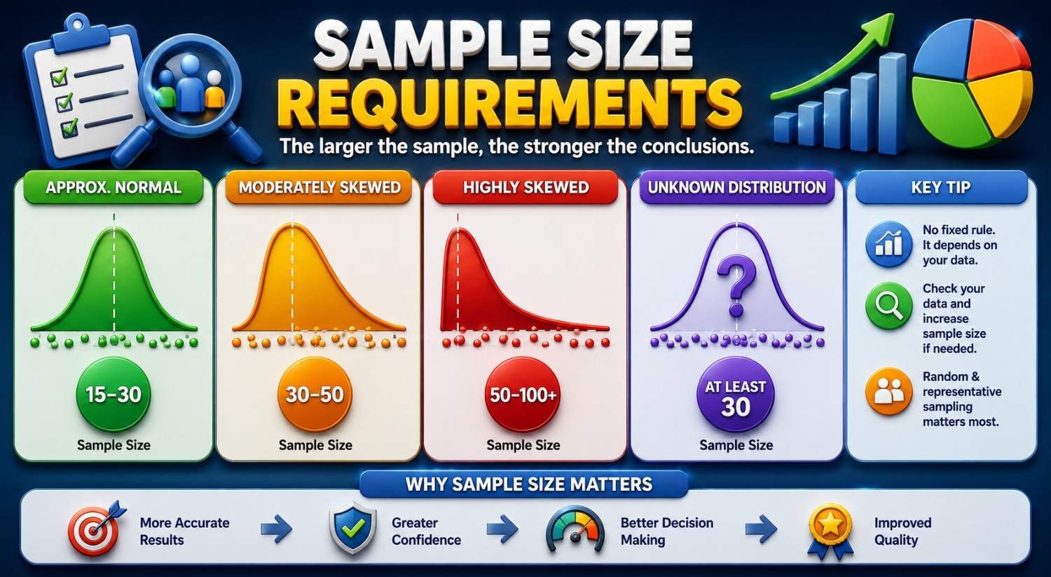
One of the most common questions about the Central Limit Theorem is "How large should the sample size be?" The answer depends on the shape of the population distribution. While 30 is widely used as a rule of thumb, it is not a universal requirement. The more the population deviates from a normal distribution, the larger the sample size generally needs to be for the sampling distribution of the mean to become approximately normal.
Why Does Sample Size Matter? As the sample size increases:
- The sampling distribution becomes more closely approximated by a normal distribution.
- The Standard Error (SE) decreases.
- Sample means become more stable and reliable.
- Confidence intervals become narrower.
- Statistical conclusions become more accurate.
Recommended Sample Sizes
Central Limit Theorem vs Law of Large Numbers
The Central Limit Theorem (CLT) and the Law of Large Numbers (LLN) are two of the most important concepts in statistics, and they're often confused because both involve increasing the sample size. I made the same mistake during my early Six Sigma training, assuming they described the same principle. It wasn't until I began analyzing real manufacturing data that I realized they answer two very different questions.
The Law of Large Numbers focuses on accuracy. It states that as the sample size increases, the sample mean gets closer to the true population mean. Simply put, collecting more observations improves the reliability of your estimate.
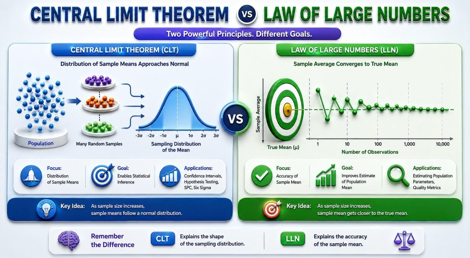
On the left side, the Law of Large Numbers is illustrated using a running average. Initially, the values fluctuate significantly, but as more observations are added, the average begins to stabilize and gradually converges toward the true population mean. This demonstrates how increasing data size improves accuracy and reliability.
On the right side, the Central Limit Theorem is represented through a histogram of sample means. Even though the original data may not follow a normal distribution, the distribution of sample averages forms a smooth, bell-shaped curve. This highlights the key idea that sample means tend to follow a normal distribution when the sample size is sufficiently large.
I often saw both principles working together during process capability studies. As we increased the number of measurements, the calculated average became more stable—demonstrating the Law of Large Numbers. At the same time, the averages from repeated samples formed the familiar bell-shaped distribution used by statistical software—illustrating the Central Limit Theorem. Seeing these concepts in practice made it much easier to understand that they complement each other rather than compete. A simple way to remember the difference is this: the Law of Large Numbers tells you that larger samples improve the accuracy of your estimate, while the Central Limit Theorem explains why those sample averages follow a predictable normal distribution. Together, these two principles form the foundation of statistical inference and modern data analysis.
📊Central Limit Theorem Calculator
Use this calculator to understand how sample size affects the sampling distribution of the mean. Enter the population mean, standard deviation, and sample size to calculate the standard error, confidence range, and Z-score.
🚀 How to Use This Calculator📊
1️⃣ Enter the Population Mean (μ) and Population Standard Deviation (σ).
2️⃣ Enter the Sample Size (n) you want to analyze.
3️⃣ Optionally enter a Sample Mean (x̄) if you would like to calculate a Z‑Score.
4️⃣ Click Calculate CLT Results to see the Sampling Distribution Mean, Standard Error, 95% Confidence Range, and Z‑Score.
💡 Example: μ = 100 | σ = 12 | n = 36 | x̄ = 104
🚗 Case Study: Engine Performance Analysis in the Automotive Industry
A leading automobile manufacturer produces engines for passenger vehicles. One critical performance parameter is fuel efficiency (km/l), which must remain consistent across all vehicles to meet regulatory standards and customer expectations.
Before a new engine design is released to the market, the quality team must verify that the manufacturing process consistently produces engines meeting the target fuel efficiency of 20 km/L.
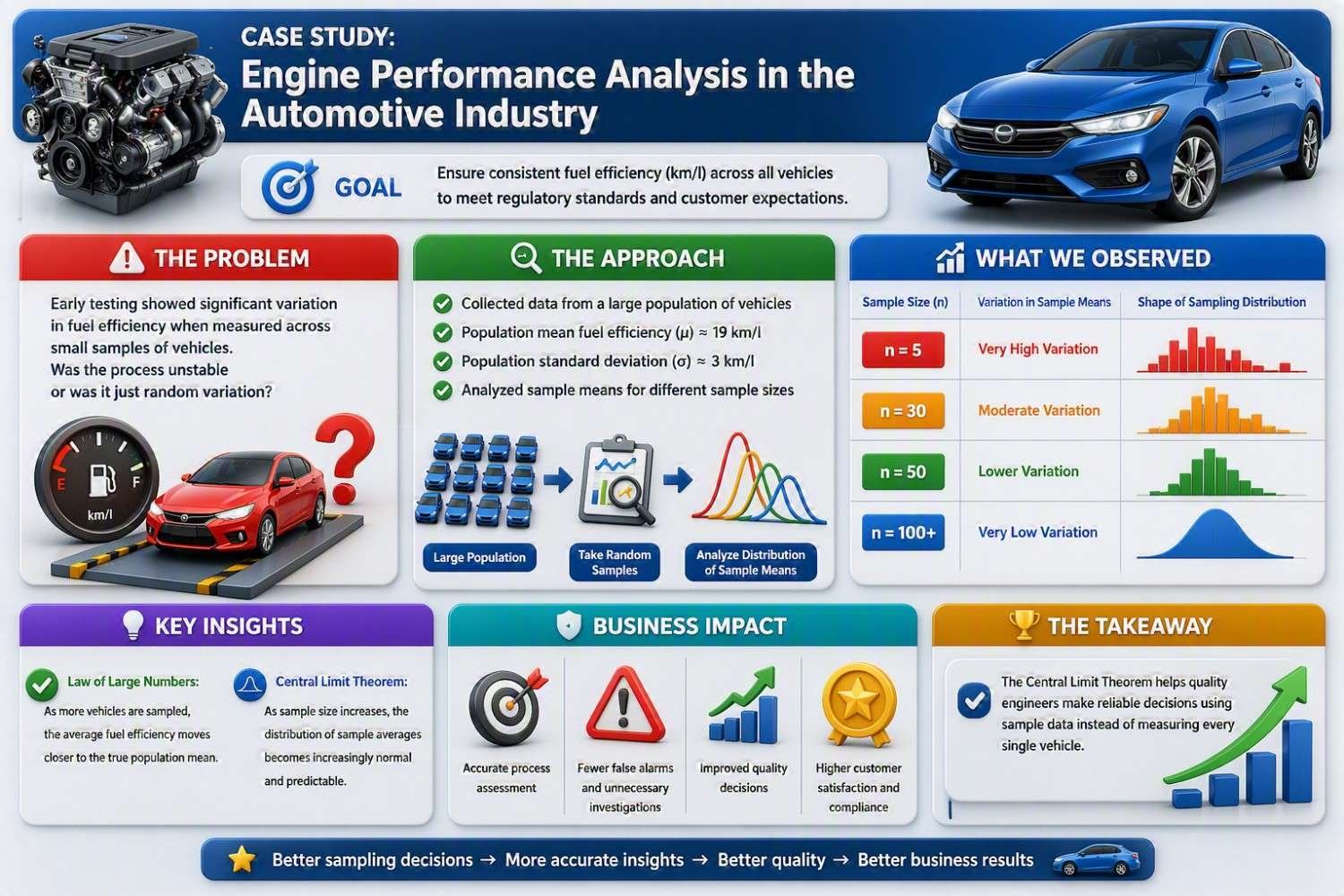
Problem: During pilot production, engineers tested a small number of vehicles from each production batch. Although the manufacturing process appeared stable, the measured fuel efficiency varied considerably. For example:
| Vehicle | Fuel Efficiency (km/L) |
|---|---|
| 1 | 18.9 |
| 2 | 20.8 |
| 3 | 19.5 |
| 4 | 21.2 |
| 5 | 19.1 |
The average looked acceptable, but every new sample produced a slightly different result. Some samples averaged 19.4 km/L, while others averaged 20.6 km/L. This raised an important question:
Was the manufacturing process actually unstable, or was this simply natural sampling variation?
Replacing equipment or adjusting the production process based on a few random observations could cost millions of dollars. The engineers needed a reliable way to separate normal variation from real process problems.
Applying the Central Limit Theorem
Instead of evaluating individual vehicle measurements, the quality team decided to analyze sample averages. They randomly selected 30 vehicles from the production line, calculated the average fuel efficiency, and repeated the sampling process hundreds of times using historical production data. Something interesting happened.
Although the fuel efficiency of individual vehicles was somewhat scattered, the distribution of the sample averages formed an almost perfect bell-shaped curve. This is exactly what the Central Limit Theorem predicts.
Because the sample means followed a normal distribution:
- Engineers could calculate confidence intervals.
- They could estimate the true average fuel efficiency of all engines.
- They could determine whether observed differences were statistically significant.
- They avoided making unnecessary process adjustments based on random fluctuations.
The Outcome
Using the Central Limit Theorem, the engineering team concluded that the observed variation was expected sampling variation, not evidence of an unstable manufacturing process.
As a result, they:
- Continued production without unnecessary machine adjustments.
- Reduced false quality investigations.
- Improved confidence in process capability studies.
- Used the results to support regulatory documentation and production approval.
Instead of reacting to every small fluctuation, the team relied on statistical evidence to make informed engineering decisions.

Lean Six Sigma • Six Sigma • Statistics • Project Management • Artificial Intelligence (AI) • Operations Management • Quality Management
FAQ on Central Limit Theorem
Why is the Law of Large Numbers important?
It ensures that larger samples produce more accurate and reliable estimates of population parameters.
Why is the Central Limit Theorem important?
It allows statisticians to use normal distribution methods even when population data is not normally distributed
Does CLT require a large sample size?
Yes—typically a sample size of around 30 or more is considered sufficient for approximation
Does LLN work for small samples?
No—LLN applies only in the long run; small samples can show large deviations from the true mean
What type of data do CLT and LLN apply to?
Both generally apply to independent and identically distributed (i.i.d.) random variables
Can CLT work even if population distribution is skewed?
Yes—the sample mean distribution still tends toward normal for large samples
How are CLT and LLN related?
LLN ensures the average stabilizes, while CLT describes how those averages are distributed.
What does LLN say about repeated experiments?
It states that repeating an experiment many times makes the average outcome closer to the expected value.
What does CLT focus on in statistics?
CLT focuses on how the distribution of sample means behaves as the sample size increases.
Why do statisticians rely on sample means?
Because LLN ensures they become more accurate estimates as sample size grows.
What happens to variability as sample size increases?
Variability decreases, making estimates more stable and reliable.
Does CLT apply to proportions as well?
Yes—CLT also works for sample proportions when the sample size is sufficiently large.
Why is independence important in CLT and LLN?
Independence ensures that each observation does not influence others, keeping results unbiased.
What is meant by “convergence” in LLN?
It refers to the sample mean getting progressively closer to the population mean.
What shape does CLT predict for large samples?
It predicts a bell-shaped (normal) distribution for sample means.
Do LLN and CLT apply only to averages?
They mainly focus on averages, but the concepts extend to other statistics as well
What happens if sample size is too small?
Results can be highly variable and may not represent the true population accurately.
How does CLT help in hypothesis testing?
It allows use of normal distribution to calculate probabilities and test assumptions.
What is a real-world example of LLN?
In manufacturing, more product samples give a better estimate of defect rates.
What is a real-world example of CLT?
In surveys, sample averages tend to follow a normal distribution even if responses are skewed.
Can CLT and LLN be used together?
Yes—LLN ensures accuracy of estimates, while CLT helps model their distribution.
Why are CLT and LLN fundamental in data analysis?
They provide the foundation for making reliable decisions based on sample data.
Continue Your Learning Journey
Learning is a continuous process. Explore related topics, practical guides, tools, calculators, templates, and learning resources to expand your knowledge and develop new skills.
Choose a category below to explore practical tutorials, tools, calculators, templates, case studies, and learning resources.
Recommended Learning Resources
Expert-led courses to build practical skills, earn credentials, and advance your career.
Recommended professional books, certification guides, and practical study resources.
Ready-to-use templates, checklists, guides, and workbooks for practical applications.
Interactive calculators for statistics, quality, engineering, analysis, and decision-making.
Interactive Z, t, Chi-Square, and F tables with critical values and distribution curves.
Discover practical tutorials, case studies, and professional resources across Quality, Lean Six Sigma, Project Management, Statistics, AI, and Data Analytics.
Published: February 10, 2025
Last Updated: September 15, 2026