What is a Confidence Interval in Statistics? How to Interpret It Correctly (With Real-World Examples & Calculator)

Why Confidence Intervals Matter

Early in my career as a Quality Engineer, I often compared processes using only the average value. If one process had a lower defect rate or a faster cycle time, it seemed obvious that it was better. But after working on several manufacturing improvement projects, I realized that averages tell only part of the story. Two processes can have almost identical averages yet differ greatly in how reliable those results are. That was when confidence intervals became one of the most valuable statistical tools in my toolbox.

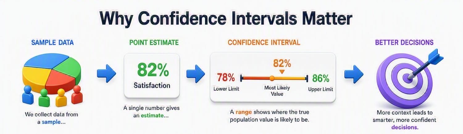
A confidence interval adds context to an estimate by showing the range within which the true population value is likely to fall. Instead of treating a sample result as an absolute fact, it acknowledges the natural variation that exists in real-world data. This simple idea helps prevent overconfidence and leads to more informed, evidence-based decisions.

Whether you’re evaluating a manufacturing process, analyzing survey results, validating a medical device, or running an A/B test, confidence intervals help answer an important question: Can I trust this result enough to make a decision? In my experience, asking that question before acting on the data has prevented far more mistakes than relying on averages alone.

What is Confidence Intervals in Statistics

I’ve learned from years of working in Quality Engineering is that an average never tells the whole story. Early in my career, I often compared processes using only the average cycle time or defect rate. It seemed like the obvious way to decide which process performed better. But after reviewing more production data, I realized that similar averages can lead to very different conclusions depending on how much uncertainty exists in the data.

A confidence interval is a range of values calculated from a sample that estimates where the true population value is likely to lie. Instead of treating a sample result as an exact answer, it acknowledges that every sample contains natural variation. In other words, it tells you how much confidence you can place in your estimate, not just what the estimate is.

I still remember a project where two manufacturing processes produced nearly identical average results. At first, they appeared equally capable. However, once I calculated the confidence intervals, one process showed much more consistent performance while the other revealed far greater variability. That single analysis changed our decision and reinforced a principle I still follow today: never rely on an average without understanding its uncertainty.

Whether you’re analyzing manufacturing data, survey results, clinical studies, or business metrics, confidence intervals provide the context that a single number cannot. They don’t remove uncertainty—they help you measure it, making your conclusions more reliable and your decisions more informed.

Why Confidence Intervals Matter

Early in my career, I would compare cycle times or defect rates and assume the lower average represented a real improvement. That changed after a process validation project where the averages looked promising, but the confidence intervals told a different story. The improvement wasn’t as certain as it first appeared, and collecting more data ultimately saved us from making the wrong decision.

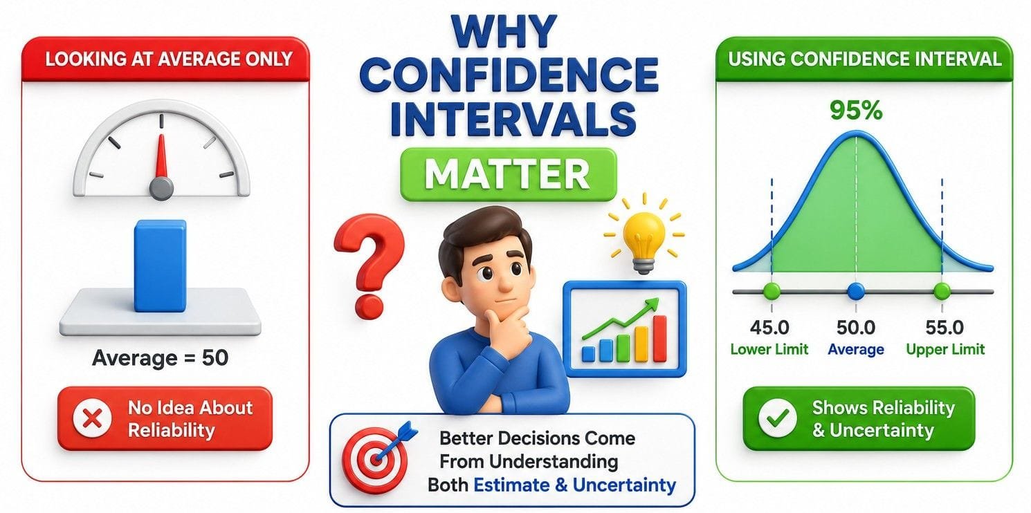
That’s why confidence intervals matter. They add the context that a single number cannot provide. Instead of asking only “What is the average?”, they answer the more important question: “How reliable is this result?” By accounting for the natural variation in sample data, confidence intervals help distinguish genuine improvements from changes that may simply be due to chance.

I now treat confidence intervals as an essential part of every data review, whether it’s a manufacturing study, a customer survey, or a Six Sigma project. They’ve taught me that good decisions aren’t based on impressive numbers alone—they’re based on understanding how much confidence those numbers deserve. That simple mindset has helped me make better decisions and avoid conclusions that the data couldn’t truly support.

Key Components of a Confidence Interval

When people first learn about confidence intervals, they often focus on the final range shown in the result and overlook what actually creates that range. In reality, every confidence interval is built from a few core statistical ingredients that work together like pieces of a puzzle. Understanding these components is more important than memorizing formulas because it helps you interpret results correctly and recognize whether the conclusions are truly reliable.

Before learning about confidence intervals, it’s important to understand what statisticians mean by an estimate. In everyday life, we make estimates all the time. We estimate how long a journey will take, how much a project might cost, or whether we have enough time to finish a task before a deadline. These estimates help us make decisions, even though we don’t know the exact answer.

The same idea applies in statistics. An estimate is a value calculated from sample data that is used to approximate an unknown population parameter. Since collecting data from an entire population is often impractical, we rely on a sample to make our best estimate of the true value.

From my experience in Quality Engineering, I rarely have the opportunity to inspect every product or analyze every measurement produced by a manufacturing process. Instead, decisions are based on carefully selected samples. The sample average provides a useful estimate, but it is still only an approximation. That’s exactly why confidence intervals are so important—they add a measure of reliability to that estimate rather than asking us to trust a single number on its own.

In statistics, estimates are broadly classified into two types: Point Estimates and Interval Estimates. Understanding the difference between these two concepts makes confidence intervals much easier to understand.

Point Estimate and Interval Estimate :

Point Estimate

A point estimate is simply a single value calculated from a sample that is used to estimate an unknown population parameter. In other words, it is our best guess of the true population value based on the information available. The simplest way to estimate an unknown population value is to calculate a single number from a sample. For example, imagine you want to estimate the average weight of employees in a large company. Weighing every employee may not be practical, so you randomly select 100 employees and calculate their average weight. If the sample average is 60 kg, then 60 kg is the point estimate of the population’s average weight.

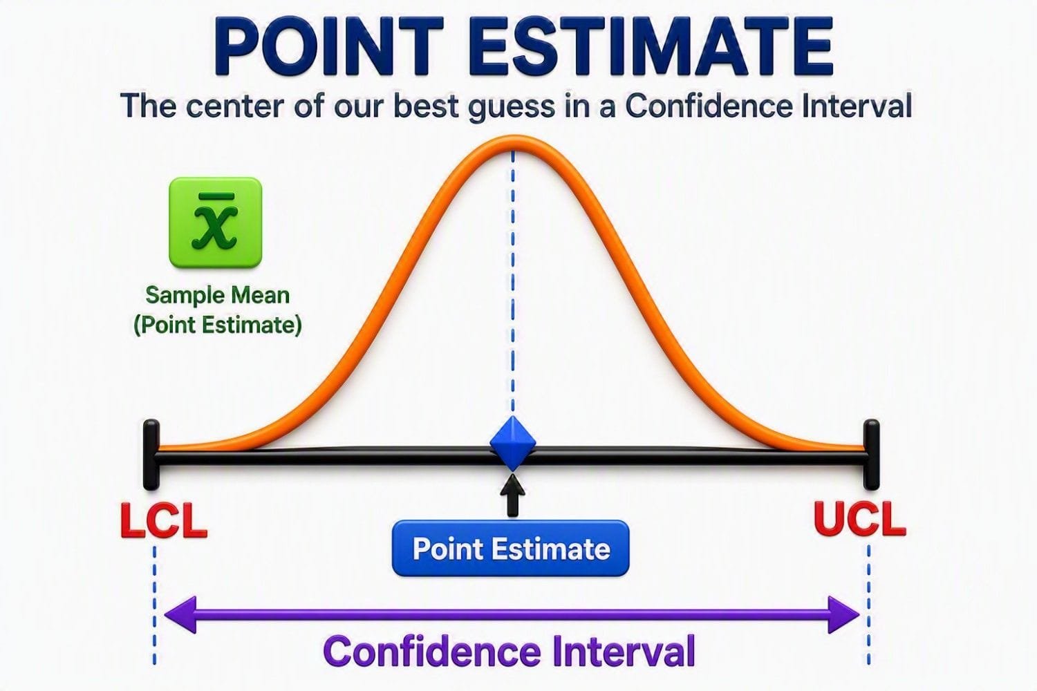
In my experience, this is where many people stop. They report the average and assume it tells the complete story. But a point estimate has one major limitation—it doesn’t tell you how reliable that estimate is. Because the estimate is based on only one sample, it is almost never exactly equal to the true population value. If you selected a different group of 100 employees, you would likely obtain a different average due to sampling error. The real question isn’t whether the estimate is right or wrong; it’s how close it is to the true population value.

For instance, if the actual population mean is 62 kg, then a sample estimate of 60 kg is reasonably close. However, if the true mean is 90 kg, the same estimate would be far less useful. A point estimate alone gives you no way to judge this uncertainty.

Interval Estimate

Because a point estimates is a single value, we can’t really tell how good it represents the population. So in inferential statistics, we prefer to use an interval or a range of values to estimate the population parameter. It gives you the range of values by calculating two different numbers between which we can expect the parameter to lie. Statisticians prefer an interval estimate rather than relying solely on a single value. An interval estimate provides a range of plausible values for the population parameter. Instead of saying the average weight is exactly 60 kg, we might say it is likely between 55 kg and 65 kg.

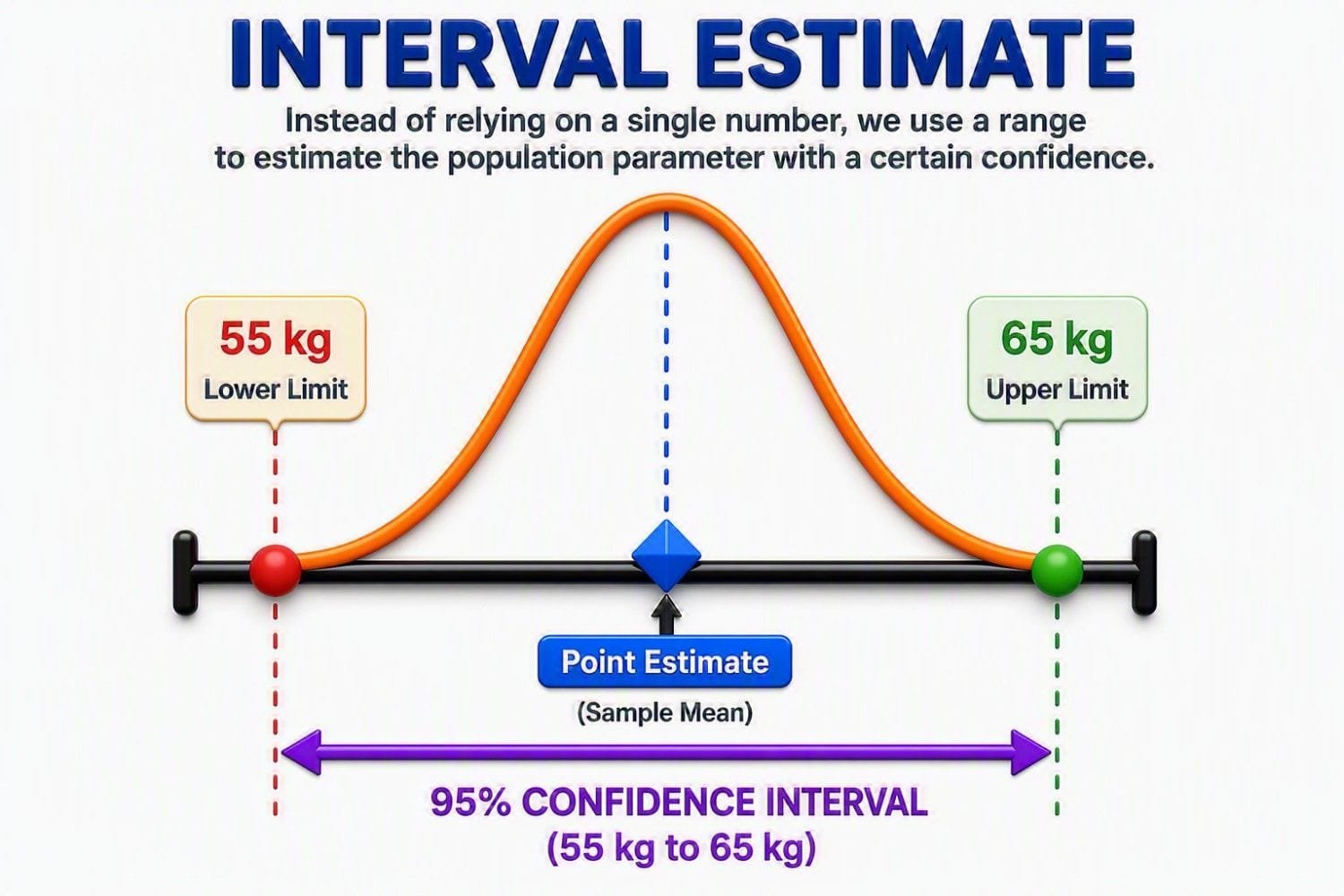
I often explain this to project teams using a simple analogy. A point estimate is like aiming at a target and reporting where you think the center is. A confidence interval tells you how much confidence you should have that the true center lies within a certain range around your estimate. For example, a 95% confidence interval means that if we repeated the same sampling process many times, approximately 95 out of 100 intervals would contain the true population value.

This shift from a single number to a range is what makes inferential statistics so powerful. Rather than pretending our estimate is exact, confidence intervals communicate both the estimate and the uncertainty surrounding it, helping us make smarter and more trustworthy decisions based on data.

Confidence Interval

One of the most common misconceptions I’ve come across is that confidence interval and confidence level mean the same thing. They don’t. The confidence level is the percentage you choose—such as 90%, 95%, or 99%—while the confidence interval is the range of values calculated from your sample. Simply put, the confidence level determines how confident you want to be, and the confidence interval is the range of values you obtain.

In simple terms, a confidence interval is the range of estimates we make for an unknown population parameter. Instead of relying on a single value, it provides both a lower limit and an upper limit, giving us a realistic range within which the true population value is likely to lie.

The relationship is straightforward:

Confidence Interval = Point Estimate ± Margin of Error

This means the point estimate is placed at the center of the interval, while the margin of error determines how far the interval extends on either side. A smaller margin of error produces a narrower, more precise interval, whereas a larger margin of error results in a wider interval, reflecting greater uncertainty.

When I first started using statistical methods in manufacturing projects, I focused mainly on the sample average. Over time, I realized that the average alone rarely answered the most important question: “How precise is this estimate?” Confidence intervals gave me that missing perspective. Instead of presenting a single number with false certainty, they helped me communicate both the estimate and the uncertainty behind it, leading to better discussions and more informed decisions.

What Does a 95% Confidence Interval Mean?

The phrase “95% confidence interval” is one of the most widely used—and most misunderstood—terms in statistics. A 95% confidence interval means that if the same study were repeated many times using the same sampling method, about 95 out of every 100 confidence intervals would contain the true population parameter. The confidence applies to the method, not to a single interval that has already been calculated.

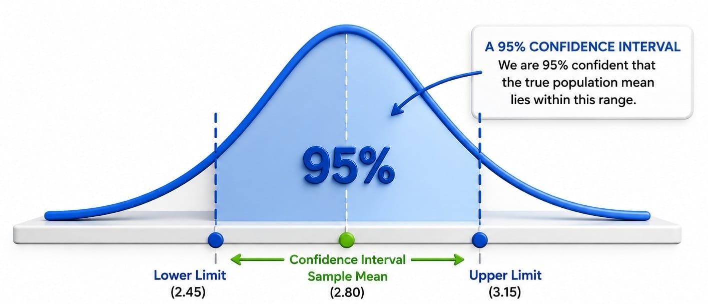
I first appreciated this while reviewing manufacturing data from different production batches. The sample averages changed slightly from batch to batch, but the confidence intervals consistently reflected the uncertainty in those estimates. That experience taught me to stop asking, “Is this average correct?” and start asking, “How reliable is this estimate?”

In most engineering, business, and research applications, 95% is the preferred confidence level because it provides a practical balance between precision and reliability. The key takeaway is simple: a 95% confidence interval doesn’t guarantee that your interval contains the true value—it tells you that the method used to construct the interval is reliable enough to capture the true value about 95% of the time over many repeated samples.

How to Calculate a Confidence Interval

To compute a confidence interval, follow these steps:

Step 1: Identify the Sample Data

Start by identifying the key information from your sample:

• Sample Mean ($\bar{x}$xˉ) or Sample Proportion ($p$p)
• Sample Standard Deviation ($s$s)
• Sample Size ($n$n)

For example, suppose a sample of 100 people has an average weight of 60 kg.

Step 2: Select the Confidence Level

The confidence level determines how confident you want to be that the interval captures the true population value.

These Z-values are used when the population standard deviation is known or the sample size is sufficiently large. For smaller samples with an unknown population standard deviation, use the t-distribution instead. In most statistical analyses, business studies, and Lean Six Sigma projects, 95% confidence is the most commonly used level.

Step 3: Calculate the Standard Error (SE)

The standard error measures the variability of the sample estimate.

The standard error measures the variability of the sample estimate.

For estimating a population mean:$$SE = \frac{s}{\sqrt{n}}$$

For estimating a population proportion:$$SE = \sqrt{\frac{p(1-p)}{n}}$$

A smaller standard error indicates a more precise estimate.

Step 4: Compute the Margin of Error (MOE)

The margin of error determines how far the confidence interval extends above and below the point estimate.
$$$$MOE=Z×SE

Where: SE = Standard Error and Z = Critical value corresponding to the chosen confidence level

Step 5: Determine the Confidence Interval

Finally, add and subtract the margin of error from the point estimate:

$$CI = \text{Point Estimate} \pm MOE$$

or$$CI = \bar{x} \pm MOE$$

This gives:$$\text{Lower Limit} = \bar{x} – MOE$$$$\text{Upper Limit} = \bar{x} + MOE$$Formula Summary

$$\boxed{CI = \text{Point Estimate} \pm (Z \times SE)}$$This simple formula is the foundation of confidence interval calculations and is widely used in statistics, market research, healthcare studies, manufacturing, and Lean Six Sigma projects to quantify uncertainty and improve decision-making.

Solved Examples:

Example 1 : CI for Single population Mean

A random sample of n = 50 males showed a mean average daily intake of dairy products equal to 756 grams with a standard deviation of 35 grams.  Find a 95% and 99% confidence interval for the population average U ? 

Ans: x ̄ = 756 grams ; n= 50 , σ = 35 ,

The Z-value can be derived from the table and its shows us which area is contained in the confidence interval of our result so in case of the 95% confidence interval we take although use between minus 1.96 times and plus 1.96 times the standard deviation. A lower confidence interval will lead to a lower Z-value and a smaller interval and vice versa.

From Z table for 95 % confidence interval we get value as 1.96.

$$\boxed{CI = \text{Point Estimate} \pm (Z \times SE)}$$

 => Interval estimate is = 756±1.96×35/√50

 => 746.30 ≤ m ≤ 765.70 grams  for 95 % confidence interval

Now for 99 % confidence interval and From Z table for 99 % CI we get value as 2.576

=> 756±2.576×35/√50

=> 743.23 ≤m≤ 768.77 grams  for 99 % confidence interval.

Example 2 : CI for Single population Proportion

Billing statement for 1000 patients discharged from a particular hospital were randomly selected for error. Out of 1000 billing statements, 102 were found to contain errors. Using this formation lets construct 99% confidence interval ?

Ans: p ̂ = 102 / 1000 = 0.102

From Z table for 99 % confidence interval we get value as 2.576

Standard Error

$$SE=\sqrt{\frac{\hat{p}(1-\hat{p})}{n}}$$$$SE=\sqrt{\frac{0.102(1-0.102)}{1000}}$$$$SE=0.00957$$Margin of Error

$$MOE=2.576 \times 0.00957$$$$MOE=0.0247$$

Confidence Interval

$$0.102 \pm 0.0247$$$$(0.0773,\;0.1267)$$

Final Answer

Confidence Interval Calculator:

Use this free Confidence Interval Calculator to estimate the range within which the true population mean or proportion is likely to fall based on sample data. Simply enter your sample statistics, select a confidence level, and instantly calculate the confidence interval, margin of error, standard error, interval width, and lower and upper confidence limits.

Note: This calculator provides statistical estimates based on the information entered. Results should be interpreted alongside subject-matter knowledge, data quality considerations, and the assumptions underlying confidence interval calculations.

Frequently Asked Questions (FAQ)

What is a confidence interval?
It is a range that estimates a population parameter based on sample data.

Why is 95% confidence most common?
It offers a practical balance between accuracy and precision.

Does a higher confidence level mean better accuracy?
Not necessarily—it increases certainty but widens the interval.

How does sample size affect confidence intervals?
Larger samples produce narrower and more reliable intervals.

Where are confidence intervals used in real life?
They are used in surveys, research studies, business forecasting, and quality improvement.

What does 95% confidence interval mean?
95% CI means that there's a 95% chance that the true mean is within the range. Larger sample size will result in a narrower confidence interval. 

Conclusion

Confidence intervals are one of the most valuable tools in statistics. They move us beyond single-point estimates and provide a realistic understanding of uncertainty. Whether you are analyzing customer data, running a Six Sigma project, or interpreting survey results, confidence intervals help you make smarter, data-driven decisions.

By understanding both the concept and application of confidence intervals, you gain a powerful advantage in interpreting and using data effectively.Confidence intervals are a vital statistical tool for estimating population parameters with a degree of certainty. By understanding their calculation, interpretation, and application, you can make more informed decisions in various fields. Mastering CIs enhances analytical skills and aids in making data-driven conclusions.

For questions please leave them in the comment box below and I’ll do my best to get back to those in a timely fashion. And remember to subscribe to Digital eLearning YouTube channel to have our latest videos sent to you while you sleep.

I hope this blog helped in understanding the basic concept in a simplified manner, watch out for I hope this blog helped in understanding the basic concept in a simplified manner, watch out for I hope this blog helped in understanding the basic concept in a simplified manner, watch out for more such stuff in the future.

📚 Where should I go after learning this concept in Statistics ?

Now that you've learned this statistical concept, the next step is building a deeper understanding of how statistics helps transform data into meaningful insights and better decisions. On Digital E-Learning, you can continue your learning journey with these related Statistics guides:

• Descriptive statistics Vs Inferential statistics
• Central Limit Theorem & Law of large numbers
• Confidence Intervals
• Sampling in Statistics
• Scales of Measurement in Statistics 

🎥 Prefer video learning?

You can also watch easy-to-understand tutorials, practical examples, and step-by-step explanations of Statistics concepts on the Digital E-Learning YouTube Channel (https://www.youtube.com/@DigitalELearning). Video lessons are designed to complement the articles and help you visualize complex statistical concepts more effectively.

👤About the Author

Aman is the Founder of Digital E-Learning and a Quality & Continuous Improvement professional with more than 25 years of experience across the Automotive, Medical Device, Manufacturing, and Consulting industries. Throughout his career, he has led and contributed to numerous initiatives in Lean Six Sigma, Quality Engineering, Risk Management, Design Assurance, Process Improvement, Problem Solving, and Operational Excellence, helping organizations enhance quality, improve efficiency, and deliver greater customer value.

Drawing on extensive real-world industry experience, Aman focuses on simplifying complex concepts into practical, easy-to-understand learning resources. His content combines proven methodologies, industry best practices, and hands-on examples to help students, engineers, quality professionals, and business leaders apply these concepts effectively in their day-to-day work.

In addition to his professional experience, Aman is the creator of the Digital E-Learning YouTube channel, a trusted learning platform followed by over 125,000 subscribers worldwide. Through his articles and videos, he shares practical knowledge in Lean Manufacturing, Six Sigma, Quality Management, Statistics, Microsoft Excel, Project Management, and Continuous Improvement.

🏆 25+ Years Industry Experience

🎓 125,000+ YouTube Learners

📚 Practical Templates & Calculators

🌍 Serving Learners Worldwide

📧: contact@digitalelearnings.com

Published: June 18, 2021
Last Updated: July 20, 2026